Quick start¶

If you have to start using Pergola in some easy steps follow this guide.

Note

This quick start guide assumes Pergola has been previously installed, if this is not the case follow instructions in the installation section.

Sample data¶

A data set containing motion behavior from C.elegans data set is available on Zenodo.

Sample data description¶

The data set contains C. elegans motion measures derived from video recordings originally used on this work.

The sample data set consists in two folders: One named worm_speeds containing a CSV file for each of the tracked worms. From the several measures that can be found in the individual files, in this example we will use mid-body speed. The mapping folder contains the worm_speed2pergola.txt, which sets the mappings between the information represented in the worm_speed files and the pergola ontology. See mapping file and pergola ontology for a deeper description.

Get the data¶

Two download the data set from Zenodo you can use this commands:

mkdir data
wget -O- https://zenodo.org/record/1161078/files/celegans_speed_sample_data.tar.gz | tar xz -C data

Run Pergola¶

Pull Pergola image¶

Tip

If you want to install Pergola on your system instead, refer to installation documentation and skip this section.

You can obtain last Pergola version from Pergola Docker Hub repository.

docker pull pergola/pergola:latest

To launch Pergola image and mount the sample data set in the container you can type:

docker run --rm -it -v "$(pwd)":/container_wd -w /container_wd pergola/pergola:latest bash

Execution¶

You can know process the downloaded sample data with Pergola using the following command:

pergola -i ./data/worm_speeds/*.csv -m ./data/mapping/worm_speed2pergola.txt -f bedGraph -w 1 -min 0 -max 29000

The resulting files can be uploaded on a desktop browser for its visualization as explained below.

Visualization with IGV¶

Once processed with Pergola, there are several available options to visualize your behavioral data. Here, we explain how to visualize the data using IGV, see visualization section for other alternatives.

Download IGV¶

As an example, we choose the Integrative Genomics Viewer (IGV) to illustrate how to visualize data. IGV can be downloaded from here.

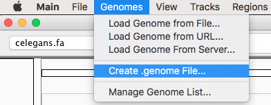
Create a genome¶

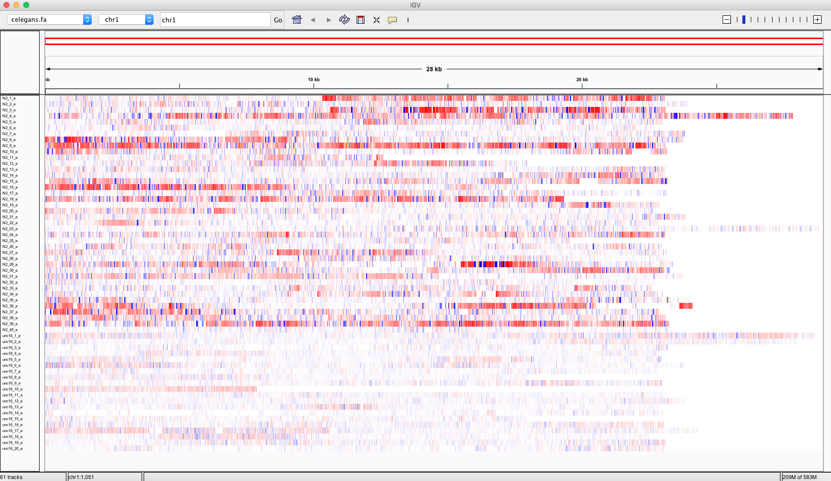
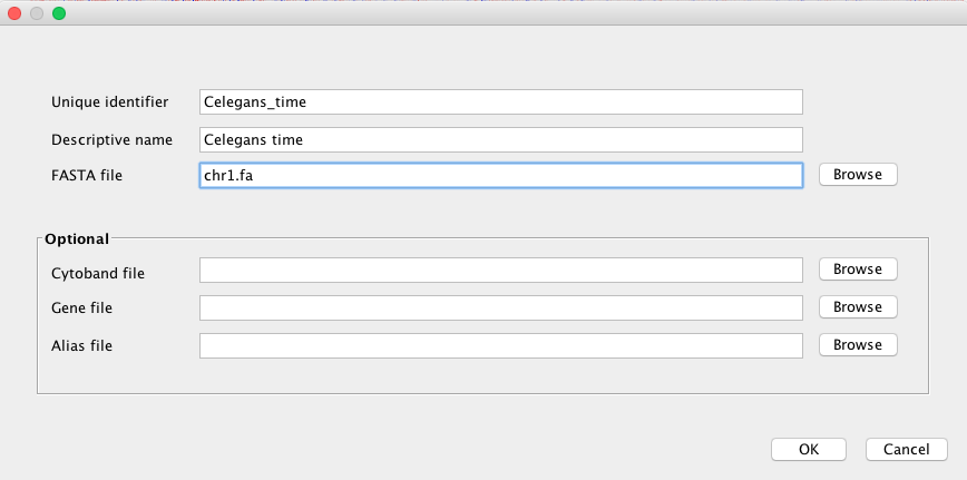
After launching IGV, first you have to create a genome file. Go to Genomes menu and click on “Create .genome File…” Data can be visualize using a heatmap.

On the menu that pops up load the fasta file generated by Pergola and click on OK.

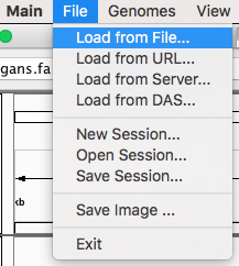
Load BedGraph files¶

Now you can render the BedGraph files generated before by going to File menu and click on “Load from File…”

Tip

Stack the tracks corresponding to each group, in this manner differences will become easier to identify

Set heatmap graphical parameters¶

Finally to obtain a heatmap of the tracks it is necessary to set some options:

To visualize all the tracks in the screen go to Tracks and click on “Fit Data to Window”

Now select all tracks by clicking on their names and right click with the mouse, as a result a menu will pop up. On this menu check “Heatmap” under Type of Graph menu and “None” under Windowing Function.

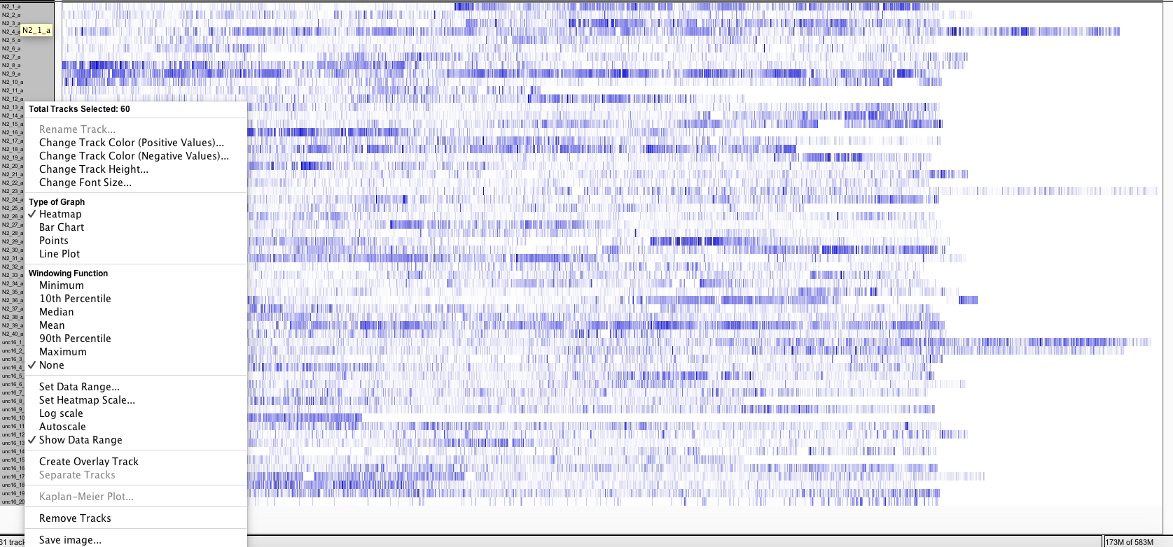
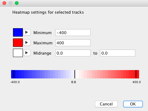
To display the differences between the tracks, adjust heatmap settings as shown in the snapshot below.

The resulting rendering shows how overall the speeds of unc-16 (uncoordinated strain), tracks below, are lower depicting a deficient moving behavior when compared to control (N2) strain on top.